Toy Grokking with a Linear Model
As a follow up to my previous post, I want to share a quick extension of understanding an implicit bias of gradient descent: we can get our toy model to grok on a properly constructed data set.
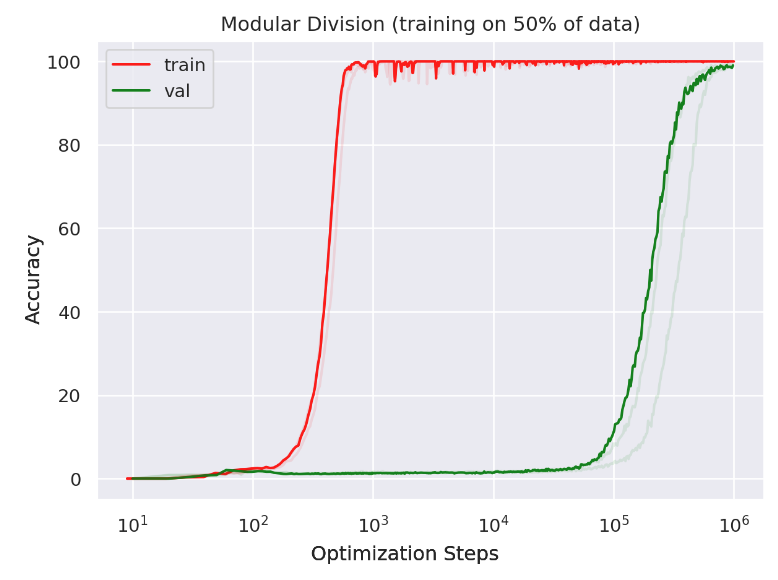
Grokking, first observed by Power et al., is characterized by an improvement from chance level to perfect generalization (measured via test accuracy), often occurring past the point of overfitting on the training set.
Here’s one story for grokking:
Our implicit biases prefers the well-generalizing (grokked) solution, but it’s also harder to learn; accordingly, we first learn the easiest solution (in this case, memorization), and then gradually evolve towards the inductive-biases-preferred solution. We do great on the test set using our inductive-biases-preferred solution, but terribly (random chance) using our easiest solution.
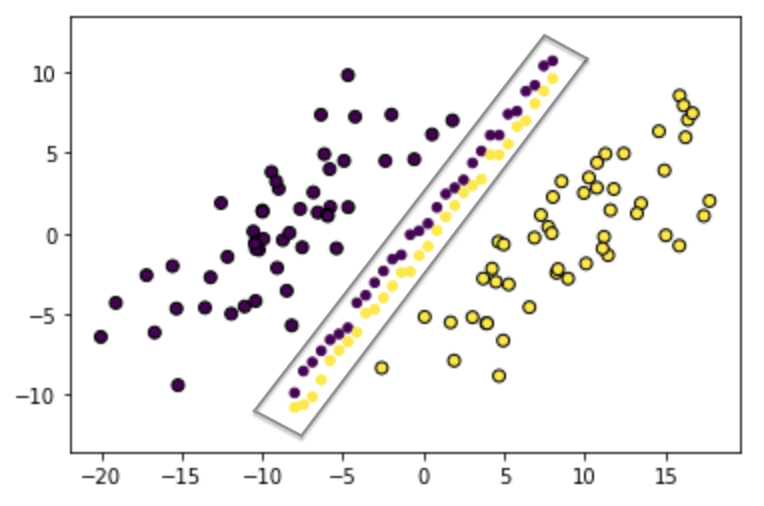
It’s pretty easy to induce this behavior in our toy setting, where we know we have an implicit bias towards the max-margin solution. Recall that we are performing binary classification on a data set of 2-dimensional points , with and . We learn a weight vector (no bias) via gradient descent on our loss function, minimizing:
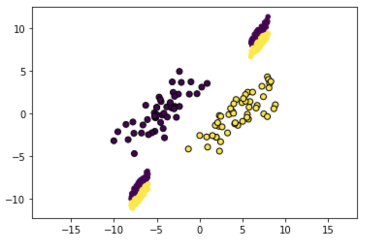
First, we construct a training data set of separable points. We then fit a hard-margin SVM to the data to find the max-margin solution, and use this to generate a test set, composed of points very close to the decision boundary (see below for visualization).
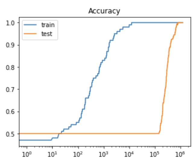
Let’s look at what happens when we train on this data (of course, only fitting to the training data):
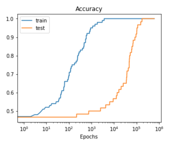
As hoped, we do see suddenly improved generalization, significantly delayed from improved train accuracy. This is because our easiest solution ends up perfectly separating the training data, while performing only slightly above chance on our test set; as our solution approaches the max-margin solution, however, we do better and better on the test set (since this is how we generated the test set in the first place).
As I emphasized in the previous post, this is due to an implicit bias (since we could also just scale up the norm of the easiest separator and still achieve arbitrarily low loss).
Loss
One interesting distinguisher between our toy case and the (also somewhat toy) Power et al. setup is the loss curves:
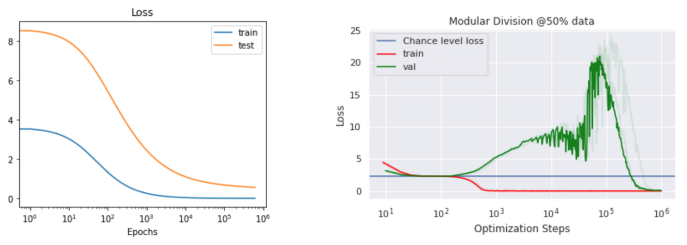
I’m not really sure why these are so different; one theory is that in our case moving from the easiest to the implicit-biases-preferred solution just means moving the decision boundary to be closer and closer to the “grokked” decision boundary (this makes the loss cleanly go down if we ignore scaling ). In more complicated (nonlinear) cases, we may follow a less straightforward path, creating a lag before our improved solution starts to benefit test performance. This effect would be compounded by an increasing weight norm, which would inflate the loss and obfuscate the improved generalization.
Conclusion
I’m not sure yet sure how much this toy grokking example has in common with the sort of grokking observed by Power et al; I do like it as a proof of concept for the easiest vs. inductive-biases-preferred framing.
One potential distinguisher that isn’t very important is the lag in generalization observed in the Power et al. case, where generalization is delayed long after perfect performance on the training set—we can make this happen in our setup by removing some of the central points, so that our test accuracy doesn’t improve until we are very close to the max-margin solution (see below).
Still, our test set is pretty clearly being sampled from a different distribution than our training set; this isn’t true in traditional grokking examples.