GD’s Implicit Bias on Separable Data
TLDR: This post goes through the intuition behind why using gradient descent to fit a linear model to linearly separable data will learn a maximum-margin decision boundary. It’s a clean example of an implicit bias of gradient descent, and also extends (in some form) to more complicated settings (like homogeneous deep networks).
Often, we use neural networks to solve optimization problems where there are many different solutions which minimize the training objective. In these cases, the particular minima we learn (or approach) is a consequence of how we go about finding a minimum; this is known as an implicit bias of our optimization algorithm. Since different global minima behave very differently outside of the training set, these implicit biases can have major effects on how our models generalize. Lots about implicit biases of different optimization algorithms still aren’t well understood; indeed, understanding these biases, and their corollary of consistently finding surprisingly well-generalizing solutions is a fundamental open problem in deep learning theory.
This post will talk about a particular setting where we do understand how this implicit bias is working. The setting is interesting not just as a toy case to develop intuition, but also because it seems like similar versions of these results may hold in much more complicated settings. It’s also useful because it forces us to confront that inductive biases are playing a role in learning; thinking only in terms of loss-minimization doesn’t explain the observed behavior.
Lots of the time I find discussion of implicit bias to be unsatisfying or confused; understanding this example well will, I hope, clear things up. Most of this math is based on “The Implicit Bias of Gradient Descent on Separable Data” by Soudry et al.
The Setting
Consider a classification data set , with d-dimensional real number inputs and binary labels We use gradient descent to find a vector which minimizes , defined by:
Our loss encourages high values of which match the sign of . We classify points according to the sign of . We assume our data is separable (that is, such that ).
With these conditions, we know that the infimum of the loss is zero, but that this can’t be achieved by any finite . We use gradient descent to minimize , with updates of the form:
With a sufficiently small , we can prove that gradient descent will converge to a global minimum as . We make no assumptions about the initialization of our weight vector .
The Task
In this setting, approaching zero loss requires the norm of to diverge to (i.e., ). However, since the sign of determines its classification, blowing up the norm of has no effect on the functional behavior of our model (and thus can’t effect things like the generalization behavior we care about).
On the other hand, the direction of our weight vector does determine classification, and thus is relevant to generalization behavior. Accordingly, we want to characterize the behavior of as . This distinction is important, and has interesting consequences like the potential for test loss to increase even as our classifier gets more accurate (we’ll talk about this in ‘Extensions’).
It’s worth focusing on the fact that a which separates the data doesn’t need to change its direction to approach a global minimum. Scaling its magnitude is enough; accordingly, we could imagine it being the case that doesn’t converge to anything in particular (and just sticks with the first separating solution it comes to while scaling up its norm). This isn’t what happens; instead, does indeed converge. I focus on this to reinforce that this result isn’t obvious, and isn’t what we come to by only reasoning about somehow getting to a global minimum.
2D Intuitive Model
There’s a really natural way to think about our setup with two dimensional points. Say we have a set of 2d points with corresponding labels .
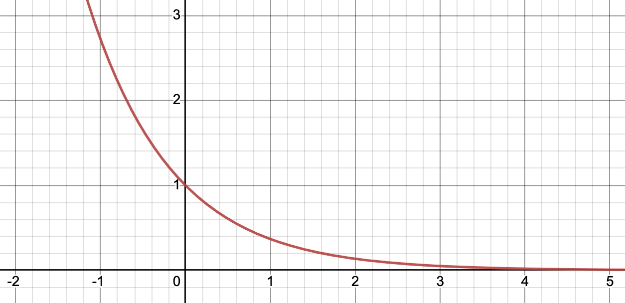
Now say . In this case, our decision boundary is the x-axis, since . Here, measures the distance between a point and the x-axis, made negative for points on the wrong side of the decision boundary. This value is then scaled according to our exponential loss, and summed to get our .
What’s cool is that we can use this same intuition for all weight vectors , since we can always decompose into a rotation () and scaling () applied to . And since , we can equivalently think about new values as performing a rotation and scaling to our data points, and then use our value to score them as a function of their distance from the x-axis (visualized below).
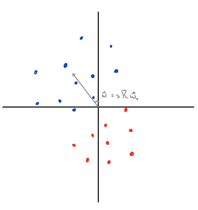
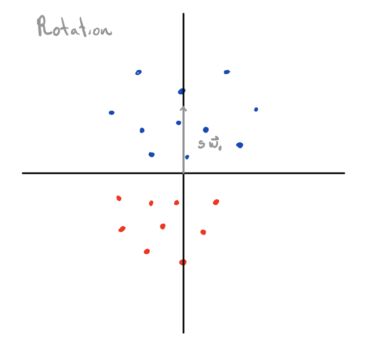
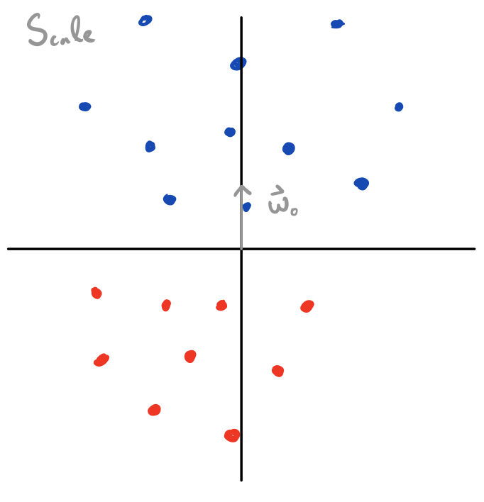
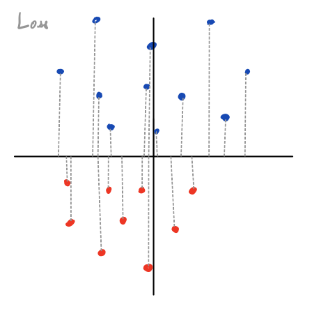
Values of which separate the data correspond to rotations which bring all points with a positive label above the x-axis, and all points with a negative label below the x axis. Scaling doesn’t change the classification, but it does change what’s plugged into , and thus our loss .
Here, any separating value of would give you zero loss if its norm was scaled to infinity; that is, every separating rotation corresponds to an (unreachable) global minimum achieved by diverging our scale to infinity. The question of implicit bias, here, is the question of which separating rotation we get among the uncountably infinite number of separating rotations (which all can tend towards global minima via scaling).
The Solution
So, what happens when we use gradient descent? How do we select between separating solutions?
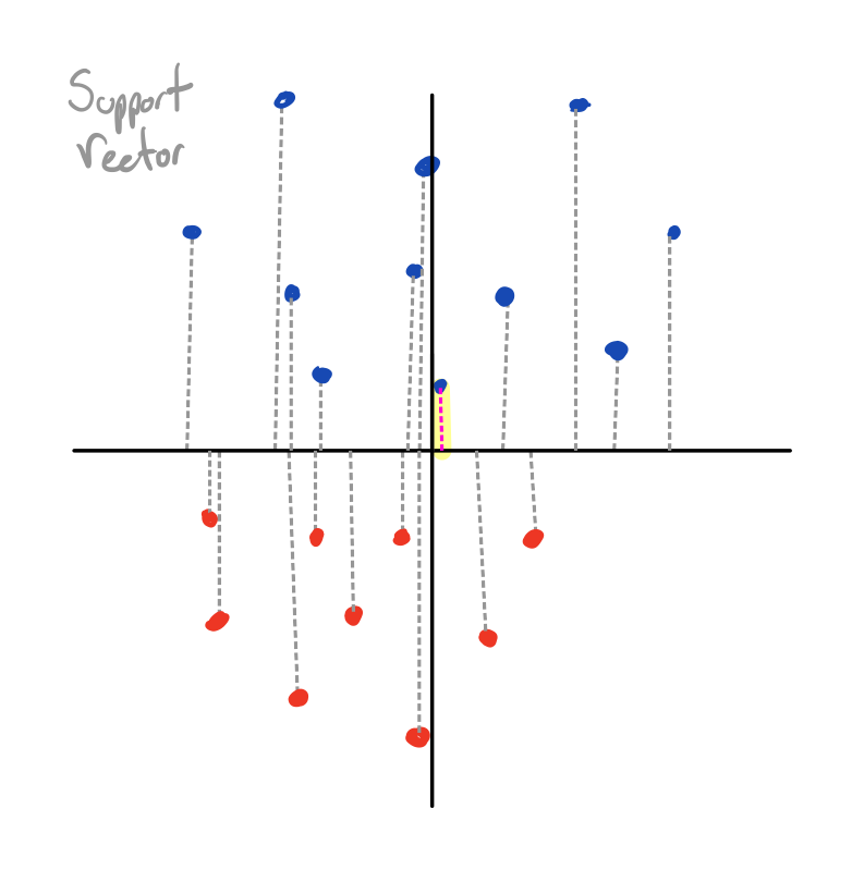
The key insight is that since , as the magnitude of diverges to infinity (as ), only the terms with the largest (least negative) exponents will meaningfully contribute to the gradient. These are the terms with the smallest margin (), which are the points closest to the decision boundary. The gradient, then, will be dominated by the closest points, scaled according to . This means that (as the magnitude of diverges to infinity), our gradient will become a linear combination of the closest points (support vectors) only.
At this point, I think it becomes intuitive that we would converge to the decision boundary preferred by these closest points, since these closest points have total control over our updates. The decision boundary preferred by these closest points, , is the max-margin solution.
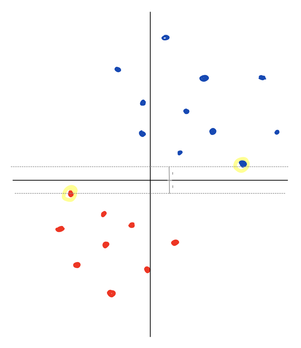
In our 2D framing, this means selecting the rotation (without scaling) which maximizes the minimum height of the points (and still correctly classifies). This is different from other plausible answers, like minimizing the sum of distances from the x-axis across all points.
One thing that’s cool is that this turns out to be the same as the direction of the with the smallest norm which maps all points to at least distance one from the decision boundary (on the correct side):
Again, this is intuitive in our 2D model; as we rotate and then attempt to scale down as much as possible, we are stopped by the points closest to the x-axis. The rotation that allows us the most scaling is the rotation which initiates these closest points furthest from the x-axis, which is the max margin solution.
It’s important to note that we only get to this solution because of the exponential tail of our loss function, since this is what made all but the support vectors’ gradients not matter.
To be (a bit) more formal, though, we can say that if converges to some value , then this must itself be dominated by a linear combination of its support vectors; the part of which does not come from these support vector gradient updates (i.e., the initial conditions) is negligible (since its norm tends to infinity). This is proportional to , which has the properties:
That is, is a combination of points distance one from the decision boundary (with the scalar’s sign corresponding to the point’s class), and all other points are further from the decision boundary. These turn out to be the KKT conditions for eq. 1, meaning is its solution. Since is proportional to , we have that does indeed converge in direction to the max-margin solution.
Extensions
This result has been extended to a broader class of loss functions (including multi-class classification with cross-entropy loss). It’s also been extended to using stochastic gradient descent, and to positive homogeneous deep networks like ReLU MLPs without bias terms. Soudry et al. expected this to be true; the below figure is taken from their paper, and shows a convolutional neural network trained on CIFAR10 using SGD.
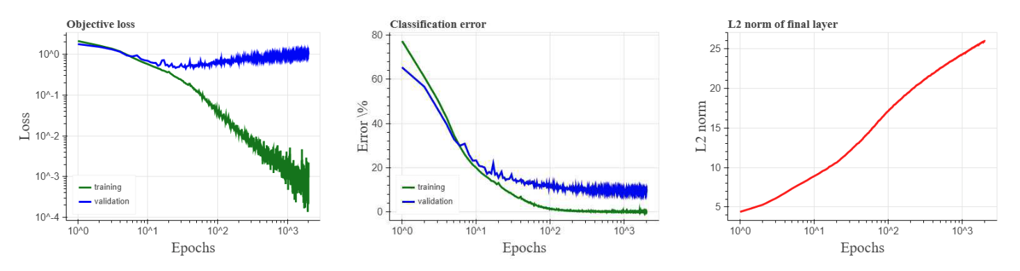
This figure initially looks weird, since the validation loss goes up as we train past separation, even as the validation accuracy improves. In light of these results, though, this is intuitive; though we are converging towards the max margin direction (which should help accuracy), we also blow up our weight norm (which amplifies any mistakes we make). Sometimes, though, we mistakenly think this increase in validation loss suggests our model is generalizing worse and worse, and decide to stop training accordingly (whereas using validation accuracy would correctly lead us to keep training).
What about adding a bias term to our original setup, learning according to ? One way to do this is to appending a one to each input, forming . Of course, our same results hold for , meaning we get the max margin solution (but in the new input space). In our 2D case, we can think of this as converting all of our points into 3D points with , and then allowing 3D rotations instead of just 2D ones. We then get the max margin solution in this 3D space.
Other Optimizers
Momentum, acceleration, and stochasticity all don’t change this implicit bias. Interestingly, though, it turns out that adaptive optimizers like Adam and AdaGrad don’t converge to the max margin predictor, and instead the limit direction can depend on the initial point and step size (though they do converge to zero loss). This might be part of the reason that these optimizers are thought to find solutions which don’t generalize as well as SGD.
Conclusion
If we understood what sorts of solutions gradient descent converged to, and what generalization properties those solutions had, we could feel more confident in predicting traits about our learned model. In particular, if we knew our model would converge to the max-margin solution of the training data, and we knew that max-margin solutions tend to generalize in particularly nice ways, we would expect our model to also generalize in nice ways (in the limit). I think this has ramifications relevant to AI safety (more info in a subsequent post), and is part of the reason I think studying the science of deep learning is useful.
Thanks to Sam Marks, Davis Brown, Hannah Erlebach, Max Nadeau, Dmitrii Krasheninnikov, and Lauro Langosco for thoughtful comments.